Machine learning is formulated as "minimization problems" of a loss function against a given set of examples (training set). This feature expresses the discrepancy between the values predicted by the model being trained and the expected values for each example instance.
The ultimate goal is to teach the model the ability to predict correctly on a set of instances not present in the training set.
A method according to which it is possible to distinguish different categories of algorithm is the type of output expected from a certain system of machine learning.
Among the main categories we find:
An example of classification is the assignment of one or more labels to an image based on the objects or subjects contained in it;
An example of regression is the estimation of the depth of a scene from its representation in the form of a color image.
In fact, the domain of the output in question is virtually infinite, and not limited to a certain discrete set of possibilities;
Linear regression is amwidely used model used to estimate real values such as:
and follows the criterion of continuous variables:
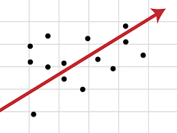
In linear regression, a relationship between independent variables and dependent variables is followed through a line that usually represents the relationship between the two variables.
The fit line is known as the regression line and is represented by a linear equation of the type Y = a * X + b.
The formula is based on interpolating data to associate two or more characteristics with each other. When you give the algorithm an input characteristic, the regression returns the other characteristic.
When we have more than one independent variable, then we speak of multiple linear regression, assuming a model like the following:
y=b0 + b1x1 + b2x2 +… + Bnxn
Basically the equation explains the relationship between a continuous dependent variable (y) and two or more independent variables (x1, x2, x3…).
For example, if we wanted to estimate the CO2 emission of a car (dependent variable y) considering the engine power, the number of cylinders and the fuel consumption. These latter factors are the independent variables x1, x2 and x3. The constants bi are real numbers and are called the model's estimated regression coefficients. Y is the continuous dependent variable, i.e. being the sum of b0, b1 x1, b2 x2, etc. y will be a real number.
Multiple regression analysis is a method used to identify the effect that independent variables have on a dependent variable.
Understanding how the dependent variable changes as the independent variables change allows us to predict the effects or impacts of changes in real situations.
Using multiple linear regression it is possible to understand how blood pressure changes as the body mass index changes by considering factors such as age, sex, etc., thus assuming what could happen.
With multiple regression we can get estimates on price trends, such as the future trend for oil or gold.
Finally, multiple linear regression is finding greater interest in the field of machine learning and artificial intelligence as it allows to obtain performing learning models even in the case of a large number of records to be analyzed.
Logistic regression is a statistical tool that aims to model a binomial result with one or more explanatory variables.
It is generally used for binary problems, where there are only two classes, for example Yes or No, 0 or 1, male or female etc ...
In this way it is possible to describe the data and explain the relationship between a binary dependent variable and one or more nominal or ordinal independent variables.
The result is determined thanks to the use of a logistic function, which estimates a probability and then defiends the closest class (positive or negative) to the obtained probability value.
We can consider logistic regression as a method of classifying the family of supervised learning algorithms.
Using statistical methods, logistic regression allows to generate a result which, in fact, represents a probability that a given input value belongs to a given class.
In binomial logistic regression problems, the probability that the output belongs to one class will be P, while that it belongs to the other class 1-P (where P is a number between 0 and 1 because it expresses a probability).
The binomial logistic regression works well in all those cases in which the variable we are trying to predict is binary, that is, it can only assume two values: the value 1 which represents the positive class, or the value 0 which represents the negative class.
Examples of problems that can be solved by logistic regression are:
With logistic regression we can do predictive analysis, measuring the relationship between what we want to predict (dependent variable) and one or more independent variables, i.e. the characteristics. Probability estimation is done through a logistic function.
The probabilities are subsequently transformed into binary values, and in order to make the forecast real, this result is assigned to the class it belongs to, based on whether or not it is close to the class itself.
For example, if the application of the logistic function returns 0,85, then it means that the input generated a positive class by assigning it to class 1. Conversely if it had obtained a value such as 0,4 or more generally <0,5 ..
Logistic regression uses the logistic function to evaluate the classification of the input values.
The logistic function, also called sigmoid, is a curve capable of taking any number of real value and mapping it to a value between 0 and 1, excluding extremes. The function is:
where:
Logistic regression uses an equation as a representation, much like linear regression
The input values (x) are linearly combined using weights or coefficient values, to predict an output value (y). A key difference from linear regression is that the modeled output value is a binary value (0 or 1) rather than a numeric value.
Below is an example of a logistic regression equation:
y = e^(b0 + b1 * x) / (1 + e^(b0 + b1 * x))
Where:
Each column in the input data has an associated b coefficient (a constant real value) that must be learned from the training data.
The actual representation of the model that you would store in memory or a file are the coefficients in the equation (the beta or b value).
Logistic regression models the probability of the default class.
As an example, let's assume we are modeling people's sex as male or female from their height, the first class could be male, and the logistic regression model could be written as the probability of being male given a person's height, or more. formally:
P (sex = male | height)
Written another way, we are modeling the probability that an input (X) belongs to the class predefinite (Y = 1), we can write it as:
P(X) = P(Y = 1 | X)
The probability prediction must be transformed into binary values (0 or 1) in order to actually make a probability prediction.
Logistic regression is a linear method, but predictions are transformed using the logistic function. The impact of this is that we can no longer understand predictions as a linear combination of inputs as we can with linear regression, for example, continuing from above, the model can be expressed as:
p(X) = e ^ (b0 + b1 * X) / (1 + e ^ (b0 + b1 * X))
Now we can reverse the equation as follows. To reverse it, we can proceed by removing the e on one side by adding a natural logarithm on the other side.
ln (p (X) / 1 - p (X)) = b0 + b1 * X
In this way we get the fact that the computation of the output on the right is linear again (just like linear regression), and the input on the left is a logarithm of the probability of the default class.
The probabilities are calculated as a ratio of the probability of the event divided by the probability of no event, e.g. 0,8 / (1-0,8) whose result is 4. So we could instead write:
ln(odds) = b0 + b1 *
Since probabilities are log-transformed, we call this left-sided log-odds or probit.
We can return the exponent to the right and write it as:
probability = e ^ (b0 + b1 * X)
All this helps us to understand that indeed the model is still a linear combination of the inputs, but that this linear combination refers to the log probabilities of the pre classdefinita.
The coefficients (beta or b values) of the logistic regression algorithm are estimated in the learning phase. To do this, we use maximum likelihood estimation.
Maximum likelihood estimation is a learning algorithm used by several machine learning algorithms. The coefficients resulting from the model predict a value very close to 1 (e.g. Male) for the pre classdefinite and a value very close to 0 (e.g. female) for the other class. Maximum likelihood for logistic regression is a procedure of finding values for coefficients (Beta or ob values) that minimize the error in the probabilities predicted by the model relative to those in the data (e.g. probability 1 if the data is the primary class).
We will use a minimization algorithm to optimize the best coefficient values for the training data. This is often implemented in practice using an efficient numerical optimization algorithm.
Developing fine motor skills through coloring prepares children for more complex skills like writing. To color…
The naval sector is a true global economic power, which has navigated towards a 150 billion market...
Last Monday, the Financial Times announced a deal with OpenAI. FT licenses its world-class journalism…
Millions of people pay for streaming services, paying monthly subscription fees. It is common opinion that you…